Covid-19 Spike Protein Example 1: Residue Neighborhoods
In this notebook, we use mdciao to analyze publicly available MD data of the Covid-19 Spike Protein, curated in the impressive COVID-19 Molecular Structure and Therapeutics Hub put together by the Molecular Sciences Software Institute (molSSI).
In particular, we use the data generated in the Chodera-Lab by Ivy Zhang, consisting of Folding@home simulations of the SARS-CoV-2 spike RBD bound to human ACE2 (725.3 µs ). We quote:
All-atom MD simulations of the SARS-CoV-2 spike protein receptor binding domain (RBD) bound to human angiotensin converting enzyme-related carboypeptidase (ACE2), simulated using Folding@Home. The “wild-type” RBD and three mutants (N439K, K417V, and the double mutant N439K/K417V) were simulated.…RUNs denote different RBD mutants: N439K (RUN0), K417V (RUN1), N439K/K417V (RUN2), and WT (RUN3). CLONEs denote different independent replica trajectories
Goals
We are going to use mdciao to compare the effect of the above mutations on the mutated residues’s vicinities or neighborhoods. This is rather simple:
Compute the residue neighborhoods for the mutated positions
N439andK417in all four datasets, using mdciao.cli.residue_neighborhoodsCompare these neighborhoods using mdciao.cli.compare for changes in the residue-residue contacts.
Residues of Interest and Molecular Topology
Since we’re not really familiar with the dataset, we can do several things to ease us into the data. Most helpful is to visualize one sample file in 3D, using the awesome nglviewer and mdtraj. We can visually inspect the setup, its components etc:
Note
A great deal of mdciao’s handling of molecular information and I/O is done using mdtraj.
[5]:
import nglview, mdtraj as md, os
datadir = "/media/perezheg/6TB_HD/FAH_aws/strided/50"
iwd = nglview.show_mdtraj(md.load(os.path.join(datadir, "run3-clone0.stride.050.h5"))[0])
iwd
Next, we’ll use mdciao’s mdciao.cli.residue_selection to locate the mutated residues in the molecular topology. Since mdciao.cli.residue_selection internally calls
mdciao.fragments.get_fragments, we also get to see how the topology is structured into chains
Note
chains isn’t really a heuristic, since the .h5 files contain chain-tags for the residues, but that will very often not be the case.
[3]:
import mdtraj as md
import nglview
import mdciao
import numpy as np
from glob import glob
import os
[4]:
datadir = "/media/perezheg/6TB_HD/FAH_aws"
for ff in sorted(glob(os.path.join(datadir, "run?-clone0*h5"))):
print("Chains for files of type:",os.path.basename(ff))
mdciao.cli.residue_selection([417,439],ff,fragments=["chains"]);
#frags = mdciao.fragments.get_fragments(ff, method="chains");
print()
Chains for files of type: run0-clone0.h5
Using method 'chains' these fragments were found
fragment 0 with 196 AAs ACE332 ( 0) - NME527 (195 ) (0)
fragment 1 with 10 AAs UYB729 ( 196) - 0fA738 (205 ) (1)
fragment 2 with 709 AAs ACE18 ( 206) - NME726 (914 ) (2)
fragment 3 with 58 AAs UYB739 ( 915) - 0fA796 (972 ) (3)
fragment 4 with 2 AAs CL973 ( 973) - ZN1 (974 ) (4) resSeq jumps
fragment 5 with 365 AAs Na+976 ( 975) - Na+1340 (1339) (5)
0.0) LYS417 in fragment 0 with residue index 85
2.0) HIS417 in fragment 2 with residue index 605
0.0) LYS439 in fragment 0 with residue index 107
2.0) LEU439 in fragment 2 with residue index 627
Your selection '[417, 439]' yields:
residue residx fragment resSeq BW CGN
LYS417 85 0 417 None None
HIS417 605 2 417 None None
LYS439 107 0 439 None None
LEU439 627 2 439 None None
Chains for files of type: run1-clone0.h5
Using method 'chains' these fragments were found
fragment 0 with 196 AAs ACE332 ( 0) - NME527 (195 ) (0)
fragment 1 with 10 AAs UYB729 ( 196) - 0fA738 (205 ) (1)
fragment 2 with 709 AAs ACE18 ( 206) - NME726 (914 ) (2)
fragment 3 with 58 AAs UYB739 ( 915) - 0fA796 (972 ) (3)
fragment 4 with 2 AAs CL973 ( 973) - ZN1 (974 ) (4) resSeq jumps
fragment 5 with 367 AAs Na+976 ( 975) - Na+1342 (1341) (5)
0.0) VAL417 in fragment 0 with residue index 85
2.0) HIS417 in fragment 2 with residue index 605
0.0) ASN439 in fragment 0 with residue index 107
2.0) LEU439 in fragment 2 with residue index 627
Your selection '[417, 439]' yields:
residue residx fragment resSeq BW CGN
VAL417 85 0 417 None None
HIS417 605 2 417 None None
ASN439 107 0 439 None None
LEU439 627 2 439 None None
Chains for files of type: run2-clone0.h5
Using method 'chains' these fragments were found
fragment 0 with 196 AAs ACE332 ( 0) - NME527 (195 ) (0)
fragment 1 with 10 AAs UYB729 ( 196) - 0fA738 (205 ) (1)
fragment 2 with 709 AAs ACE18 ( 206) - NME726 (914 ) (2)
fragment 3 with 58 AAs UYB739 ( 915) - 0fA796 (972 ) (3)
fragment 4 with 2 AAs CL973 ( 973) - ZN1 (974 ) (4) resSeq jumps
fragment 5 with 366 AAs Na+976 ( 975) - Na+1341 (1340) (5)
0.0) VAL417 in fragment 0 with residue index 85
2.0) HIS417 in fragment 2 with residue index 605
0.0) LYS439 in fragment 0 with residue index 107
2.0) LEU439 in fragment 2 with residue index 627
Your selection '[417, 439]' yields:
residue residx fragment resSeq BW CGN
VAL417 85 0 417 None None
HIS417 605 2 417 None None
LYS439 107 0 439 None None
LEU439 627 2 439 None None
Chains for files of type: run3-clone0.h5
Using method 'chains' these fragments were found
fragment 0 with 196 AAs ACE332 ( 0) - NME527 (195 ) (0)
fragment 1 with 10 AAs UYB729 ( 196) - 0fA738 (205 ) (1)
fragment 2 with 709 AAs ACE18 ( 206) - NME726 (914 ) (2)
fragment 3 with 58 AAs UYB739 ( 915) - 0fA796 (972 ) (3)
fragment 4 with 2 AAs CL973 ( 973) - ZN1 (974 ) (4) resSeq jumps
fragment 5 with 366 AAs Na+976 ( 975) - Na+1341 (1340) (5)
0.0) LYS417 in fragment 0 with residue index 85
2.0) HIS417 in fragment 2 with residue index 605
0.0) ASN439 in fragment 0 with residue index 107
2.0) LEU439 in fragment 2 with residue index 627
Your selection '[417, 439]' yields:
residue residx fragment resSeq BW CGN
LYS417 85 0 417 None None
HIS417 605 2 417 None None
ASN439 107 0 439 None None
LEU439 627 2 439 None None
Some observations:
All setups have the same overall topology, with the same six fragments/chains:
RBD (SARS-CoV-2 spike protein receptor binding domain)
ACE (human angiotensin converting enzyme-related carboypeptidase)
ions (probably crystallographic ions CL and ZN)
ions (NaCl)
We clearly identify that the residues with resSeq
417and439in the Spike-RBD have the serial indices85and107, respectively in all setups. It’s the part of the outputs that look like this:
``` 0.0) LYS417 in fragment 0 with residue index 85 2.0) HIS417 in fragment 2 with residue index 605 0.0) ASN439 in fragment 0 with residue index 107 2.0) LEU439 in fragment 2 with residue index 627 Your selection ‘[417, 439]’ yields: residue residx fragment resSeq BW CGN LYS417 85 0 417 None None HIS417 605 2 417 None None ASN439 107 0 439 None None LEU439 627 2 439 None None
Depending on the
RUNindex (0 to 3), these positions have different aminoacids (AAs) because of point mutations:run0 : N439K
run1 : K417V
run2 : N439K/K417V
run3 : WT
We can also use the RUN1,RUN2,... filename-schemes to create a dictionary assigning filenaming-schemes to a setup, as we do below with the filename2system-dictionary:
[4]:
filename2system = {
"run0" : "N439K",
"run1" : "K417V",
"run2" : "N439K/K417V",
"run3" : "WT"
}
Viewing Local Changes through Residue Neighborhoods
We now compute the residue neighborhoods around the mutated sites using mdciao.cli.residue_neighborhoods.
Since the point-mutations didn’t alter the serial indices 85 and 107 for resSeqs 417 and 439, respectively, we can use them to address these positions in all setups.
Computing the Neighborhoods
[5]:
neighborhoods = {}
for fn, syskey in filename2system.items():
pattern = os.path.join(datadir,fn+"*.h5")
ineigh = mdciao.cli.residue_neighborhoods([85,107],
pattern,
res_idxs=True,
n_jobs=7,
ctc_cutoff_Ang=4,
fragment_names=["RBD","GLY_RBD","ACE","GLY_ACE","ions","ions"],
fragments=["chains"],
ctc_control=.99,
no_disk=True,
plot_timedep=False)["neighborhoods"]
neighborhoods[syskey]=ineigh
Will compute contact frequencies for (2000 items):
/media/perezheg/6TB_HD/FAH_aws/strided/50/run0-clone0.stride.050.h5
/media/perezheg/6TB_HD/FAH_aws/strided/50/run0-clone1.stride.050.h5
/media/perezheg/6TB_HD/FAH_aws/strided/50/run0-clone2.stride.050.h5
/media/perezheg/6TB_HD/FAH_aws/strided/50/run0-clone3.stride.050.h5
/media/perezheg/6TB_HD/FAH_aws/strided/50/run0-clone4.stride.050.h5
/media/perezheg/6TB_HD/FAH_aws/strided/50/run0-clone5.stride.050.h5
/media/perezheg/6TB_HD/FAH_aws/strided/50/run0-clone6.stride.050.h5
/media/perezheg/6TB_HD/FAH_aws/strided/50/run0-clone7.stride.050.h5
/media/perezheg/6TB_HD/FAH_aws/strided/50/run0-clone8.stride.050.h5
/media/perezheg/6TB_HD/FAH_aws/strided/50/run0-clone9.stride.050.h5
/media/perezheg/6TB_HD/FAH_aws/strided/50/run0-clone10.stride.050.h5
/media/perezheg/6TB_HD/FAH_aws/strided/50/run0-clone11.stride.050.h5
/media/perezheg/6TB_HD/FAH_aws/strided/50/run0-clone12.stride.050.h5
/media/perezheg/6TB_HD/FAH_aws/strided/50/run0-clone13.stride.050.h5
/media/perezheg/6TB_HD/FAH_aws/strided/50/run0-clone14.stride.050.h5
...[long list: omitted 1970 items]...
/media/perezheg/6TB_HD/FAH_aws/strided/50/run0-clone1985.stride.050.h5
/media/perezheg/6TB_HD/FAH_aws/strided/50/run0-clone1986.stride.050.h5
/media/perezheg/6TB_HD/FAH_aws/strided/50/run0-clone1987.stride.050.h5
/media/perezheg/6TB_HD/FAH_aws/strided/50/run0-clone1988.stride.050.h5
/media/perezheg/6TB_HD/FAH_aws/strided/50/run0-clone1989.stride.050.h5
/media/perezheg/6TB_HD/FAH_aws/strided/50/run0-clone1990.stride.050.h5
/media/perezheg/6TB_HD/FAH_aws/strided/50/run0-clone1991.stride.050.h5
/media/perezheg/6TB_HD/FAH_aws/strided/50/run0-clone1992.stride.050.h5
/media/perezheg/6TB_HD/FAH_aws/strided/50/run0-clone1993.stride.050.h5
/media/perezheg/6TB_HD/FAH_aws/strided/50/run0-clone1994.stride.050.h5
/media/perezheg/6TB_HD/FAH_aws/strided/50/run0-clone1995.stride.050.h5
/media/perezheg/6TB_HD/FAH_aws/strided/50/run0-clone1996.stride.050.h5
/media/perezheg/6TB_HD/FAH_aws/strided/50/run0-clone1997.stride.050.h5
/media/perezheg/6TB_HD/FAH_aws/strided/50/run0-clone1998.stride.050.h5
/media/perezheg/6TB_HD/FAH_aws/strided/50/run0-clone1999.stride.050.h5
with a stride of 1 frames
Using method 'chains' these fragments were found
fragment 0 with 196 AAs ACE332 ( 0) - NME527 (195 ) (0)
fragment 1 with 10 AAs UYB729 ( 196) - 0fA738 (205 ) (1)
fragment 2 with 709 AAs ACE18 ( 206) - NME726 (914 ) (2)
fragment 3 with 58 AAs UYB739 ( 915) - 0fA796 (972 ) (3)
fragment 4 with 2 AAs CL973 ( 973) - ZN1 (974 ) (4) resSeq jumps
fragment 5 with 365 AAs Na+976 ( 975) - Na+1340 (1339) (5)
Will compute neighborhoods for the residues
[85, 107]
excluding 4 nearest neighbors
residue residx fragment resSeq BW CGN
LYS417 85 0 417 None None
LYS439 107 0 439 None None
Pre-computing likely neighborhoods by reducing the neighbor-list
to those within 15 Angstrom in the first frame of reference geom
'<mdtraj.Trajectory with 1 frames, 16347 atoms, 1340 residues, and unitcells>':...done!
From 2662 potential distances, the neighborhoods have been reduced to only 184 potential contacts.
If this number is still too high (i.e. the computation is too slow), consider using a smaller nlist_cutoff_Ang
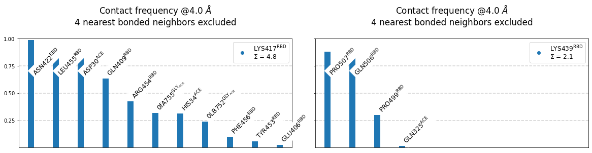
#idx freq contact fragments res_idxs ctc_idx Sum
1: 0.99 LYS417-ASN422 0-0 85-90 22 0.99
2: 0.89 LYS417-LEU455 0-0 85-123 31 1.88
3: 0.82 LYS417-ASP30 0-2 85-218 78 2.70
4: 0.64 LYS417-GLN409 0-0 85-77 18 3.33
5: 0.42 LYS417-ARG454 0-0 85-122 30 3.76
6: 0.32 LYS417-0fA755 0-3 85-931 109 4.08
7: 0.31 LYS417-HIS34 0-2 85-222 82 4.39
8: 0.24 LYS417-0LB752 0-3 85-928 107 4.63
9: 0.10 LYS417-PHE456 0-0 85-124 32 4.73
10: 0.06 LYS417-TYR453 0-0 85-121 29 4.79
11: 0.02 LYS417-GLU406 0-0 85-74 15 4.81
These 11 contacts capture 4.81 (~99%) of the total frequency 4.84 (over 111 input contacts)
#idx freq contact fragments res_idxs ctc_idx Sum
1: 0.88 LYS439-PRO507 0-0 107-175 154 0.88
2: 0.88 LYS439-GLN506 0-0 107-174 153 1.76
3: 0.30 LYS439-PRO499 0-0 107-167 146 2.06
4: 0.02 LYS439-GLN325 0-2 107-513 165 2.08
These 4 contacts capture 2.08 (~99%) of the total frequency 2.09 (over 73 input contacts)
Will compute contact frequencies for (1998 items):
/media/perezheg/6TB_HD/FAH_aws/strided/50/run1-clone0.stride.050.h5
/media/perezheg/6TB_HD/FAH_aws/strided/50/run1-clone1.stride.050.h5
/media/perezheg/6TB_HD/FAH_aws/strided/50/run1-clone2.stride.050.h5
/media/perezheg/6TB_HD/FAH_aws/strided/50/run1-clone3.stride.050.h5
/media/perezheg/6TB_HD/FAH_aws/strided/50/run1-clone4.stride.050.h5
/media/perezheg/6TB_HD/FAH_aws/strided/50/run1-clone5.stride.050.h5
/media/perezheg/6TB_HD/FAH_aws/strided/50/run1-clone6.stride.050.h5
/media/perezheg/6TB_HD/FAH_aws/strided/50/run1-clone7.stride.050.h5
/media/perezheg/6TB_HD/FAH_aws/strided/50/run1-clone8.stride.050.h5
/media/perezheg/6TB_HD/FAH_aws/strided/50/run1-clone9.stride.050.h5
/media/perezheg/6TB_HD/FAH_aws/strided/50/run1-clone10.stride.050.h5
/media/perezheg/6TB_HD/FAH_aws/strided/50/run1-clone11.stride.050.h5
/media/perezheg/6TB_HD/FAH_aws/strided/50/run1-clone12.stride.050.h5
/media/perezheg/6TB_HD/FAH_aws/strided/50/run1-clone13.stride.050.h5
/media/perezheg/6TB_HD/FAH_aws/strided/50/run1-clone14.stride.050.h5
...[long list: omitted 1968 items]...
/media/perezheg/6TB_HD/FAH_aws/strided/50/run1-clone1985.stride.050.h5
/media/perezheg/6TB_HD/FAH_aws/strided/50/run1-clone1986.stride.050.h5
/media/perezheg/6TB_HD/FAH_aws/strided/50/run1-clone1987.stride.050.h5
/media/perezheg/6TB_HD/FAH_aws/strided/50/run1-clone1988.stride.050.h5
/media/perezheg/6TB_HD/FAH_aws/strided/50/run1-clone1989.stride.050.h5
/media/perezheg/6TB_HD/FAH_aws/strided/50/run1-clone1990.stride.050.h5
/media/perezheg/6TB_HD/FAH_aws/strided/50/run1-clone1991.stride.050.h5
/media/perezheg/6TB_HD/FAH_aws/strided/50/run1-clone1992.stride.050.h5
/media/perezheg/6TB_HD/FAH_aws/strided/50/run1-clone1993.stride.050.h5
/media/perezheg/6TB_HD/FAH_aws/strided/50/run1-clone1994.stride.050.h5
/media/perezheg/6TB_HD/FAH_aws/strided/50/run1-clone1995.stride.050.h5
/media/perezheg/6TB_HD/FAH_aws/strided/50/run1-clone1996.stride.050.h5
/media/perezheg/6TB_HD/FAH_aws/strided/50/run1-clone1997.stride.050.h5
/media/perezheg/6TB_HD/FAH_aws/strided/50/run1-clone1998.stride.050.h5
/media/perezheg/6TB_HD/FAH_aws/strided/50/run1-clone1999.stride.050.h5
with a stride of 1 frames
Using method 'chains' these fragments were found
fragment 0 with 196 AAs ACE332 ( 0) - NME527 (195 ) (0)
fragment 1 with 10 AAs UYB729 ( 196) - 0fA738 (205 ) (1)
fragment 2 with 709 AAs ACE18 ( 206) - NME726 (914 ) (2)
fragment 3 with 58 AAs UYB739 ( 915) - 0fA796 (972 ) (3)
fragment 4 with 2 AAs CL973 ( 973) - ZN1 (974 ) (4) resSeq jumps
fragment 5 with 367 AAs Na+976 ( 975) - Na+1342 (1341) (5)
Will compute neighborhoods for the residues
[85, 107]
excluding 4 nearest neighbors
residue residx fragment resSeq BW CGN
VAL417 85 0 417 None None
ASN439 107 0 439 None None
Pre-computing likely neighborhoods by reducing the neighbor-list
to those within 15 Angstrom in the first frame of reference geom
'<mdtraj.Trajectory with 1 frames, 16335 atoms, 1342 residues, and unitcells>':...done!
From 2666 potential distances, the neighborhoods have been reduced to only 174 potential contacts.
If this number is still too high (i.e. the computation is too slow), consider using a smaller nlist_cutoff_Ang
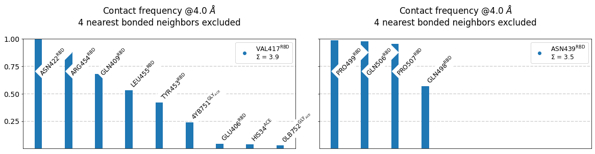
#idx freq contact fragments res_idxs ctc_idx Sum
1: 1.00 VAL417-ASN422 0-0 85-90 21 1.00
2: 0.88 VAL417-ARG454 0-0 85-122 30 1.88
3: 0.68 VAL417-GLN409 0-0 85-77 17 2.56
4: 0.53 VAL417-LEU455 0-0 85-123 31 3.10
5: 0.42 VAL417-TYR453 0-0 85-121 29 3.51
6: 0.24 VAL417-4YB751 0-3 85-927 96 3.75
7: 0.04 VAL417-GLU406 0-0 85-74 14 3.79
8: 0.04 VAL417-HIS34 0-2 85-222 78 3.83
9: 0.03 VAL417-0LB752 0-3 85-928 97 3.86
These 9 contacts capture 3.86 (~99%) of the total frequency 3.89 (over 102 input contacts)
#idx freq contact fragments res_idxs ctc_idx Sum
1: 0.99 ASN439-PRO499 0-0 107-167 138 0.99
2: 0.98 ASN439-GLN506 0-0 107-174 145 1.96
3: 0.95 ASN439-PRO507 0-0 107-175 146 2.92
4: 0.57 ASN439-GLN498 0-0 107-166 137 3.48
These 4 contacts capture 3.48 (~100%) of the total frequency 3.48 (over 72 input contacts)
Will compute contact frequencies for (2000 items):
/media/perezheg/6TB_HD/FAH_aws/strided/50/run2-clone0.stride.050.h5
/media/perezheg/6TB_HD/FAH_aws/strided/50/run2-clone1.stride.050.h5
/media/perezheg/6TB_HD/FAH_aws/strided/50/run2-clone2.stride.050.h5
/media/perezheg/6TB_HD/FAH_aws/strided/50/run2-clone3.stride.050.h5
/media/perezheg/6TB_HD/FAH_aws/strided/50/run2-clone4.stride.050.h5
/media/perezheg/6TB_HD/FAH_aws/strided/50/run2-clone5.stride.050.h5
/media/perezheg/6TB_HD/FAH_aws/strided/50/run2-clone6.stride.050.h5
/media/perezheg/6TB_HD/FAH_aws/strided/50/run2-clone7.stride.050.h5
/media/perezheg/6TB_HD/FAH_aws/strided/50/run2-clone8.stride.050.h5
/media/perezheg/6TB_HD/FAH_aws/strided/50/run2-clone9.stride.050.h5
/media/perezheg/6TB_HD/FAH_aws/strided/50/run2-clone10.stride.050.h5
/media/perezheg/6TB_HD/FAH_aws/strided/50/run2-clone11.stride.050.h5
/media/perezheg/6TB_HD/FAH_aws/strided/50/run2-clone12.stride.050.h5
/media/perezheg/6TB_HD/FAH_aws/strided/50/run2-clone13.stride.050.h5
/media/perezheg/6TB_HD/FAH_aws/strided/50/run2-clone14.stride.050.h5
...[long list: omitted 1970 items]...
/media/perezheg/6TB_HD/FAH_aws/strided/50/run2-clone1985.stride.050.h5
/media/perezheg/6TB_HD/FAH_aws/strided/50/run2-clone1986.stride.050.h5
/media/perezheg/6TB_HD/FAH_aws/strided/50/run2-clone1987.stride.050.h5
/media/perezheg/6TB_HD/FAH_aws/strided/50/run2-clone1988.stride.050.h5
/media/perezheg/6TB_HD/FAH_aws/strided/50/run2-clone1989.stride.050.h5
/media/perezheg/6TB_HD/FAH_aws/strided/50/run2-clone1990.stride.050.h5
/media/perezheg/6TB_HD/FAH_aws/strided/50/run2-clone1991.stride.050.h5
/media/perezheg/6TB_HD/FAH_aws/strided/50/run2-clone1992.stride.050.h5
/media/perezheg/6TB_HD/FAH_aws/strided/50/run2-clone1993.stride.050.h5
/media/perezheg/6TB_HD/FAH_aws/strided/50/run2-clone1994.stride.050.h5
/media/perezheg/6TB_HD/FAH_aws/strided/50/run2-clone1995.stride.050.h5
/media/perezheg/6TB_HD/FAH_aws/strided/50/run2-clone1996.stride.050.h5
/media/perezheg/6TB_HD/FAH_aws/strided/50/run2-clone1997.stride.050.h5
/media/perezheg/6TB_HD/FAH_aws/strided/50/run2-clone1998.stride.050.h5
/media/perezheg/6TB_HD/FAH_aws/strided/50/run2-clone1999.stride.050.h5
with a stride of 1 frames
Using method 'chains' these fragments were found
fragment 0 with 196 AAs ACE332 ( 0) - NME527 (195 ) (0)
fragment 1 with 10 AAs UYB729 ( 196) - 0fA738 (205 ) (1)
fragment 2 with 709 AAs ACE18 ( 206) - NME726 (914 ) (2)
fragment 3 with 58 AAs UYB739 ( 915) - 0fA796 (972 ) (3)
fragment 4 with 2 AAs CL973 ( 973) - ZN1 (974 ) (4) resSeq jumps
fragment 5 with 366 AAs Na+976 ( 975) - Na+1341 (1340) (5)
Will compute neighborhoods for the residues
[85, 107]
excluding 4 nearest neighbors
residue residx fragment resSeq BW CGN
VAL417 85 0 417 None None
LYS439 107 0 439 None None
Pre-computing likely neighborhoods by reducing the neighbor-list
to those within 15 Angstrom in the first frame of reference geom
'<mdtraj.Trajectory with 1 frames, 16342 atoms, 1341 residues, and unitcells>':...done!
From 2664 potential distances, the neighborhoods have been reduced to only 179 potential contacts.
If this number is still too high (i.e. the computation is too slow), consider using a smaller nlist_cutoff_Ang
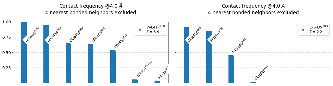
#idx freq contact fragments res_idxs ctc_idx Sum
1: 1.00 VAL417-ASN422 0-0 85-90 21 1.00
2: 0.95 VAL417-ARG454 0-0 85-122 31 1.95
3: 0.66 VAL417-GLN409 0-0 85-77 17 2.60
4: 0.64 VAL417-LEU455 0-0 85-123 32 3.24
5: 0.54 VAL417-TYR453 0-0 85-121 30 3.78
6: 0.06 VAL417-4YB751 0-3 85-927 98 3.83
7: 0.04 VAL417-HIS34 0-2 85-222 80 3.87
These 7 contacts capture 3.87 (~99%) of the total frequency 3.91 (over 106 input contacts)
#idx freq contact fragments res_idxs ctc_idx Sum
1: 0.92 LYS439-GLN506 0-0 107-174 148 0.92
2: 0.85 LYS439-PRO507 0-0 107-175 149 1.77
3: 0.45 LYS439-PRO499 0-0 107-167 141 2.22
4: 0.02 LYS439-GLN325 0-2 107-513 162 2.24
These 4 contacts capture 2.24 (~99%) of the total frequency 2.25 (over 73 input contacts)
Will compute contact frequencies for (2000 items):
/media/perezheg/6TB_HD/FAH_aws/strided/50/run3-clone0.stride.050.h5
/media/perezheg/6TB_HD/FAH_aws/strided/50/run3-clone1.stride.050.h5
/media/perezheg/6TB_HD/FAH_aws/strided/50/run3-clone2.stride.050.h5
/media/perezheg/6TB_HD/FAH_aws/strided/50/run3-clone3.stride.050.h5
/media/perezheg/6TB_HD/FAH_aws/strided/50/run3-clone4.stride.050.h5
/media/perezheg/6TB_HD/FAH_aws/strided/50/run3-clone5.stride.050.h5
/media/perezheg/6TB_HD/FAH_aws/strided/50/run3-clone6.stride.050.h5
/media/perezheg/6TB_HD/FAH_aws/strided/50/run3-clone7.stride.050.h5
/media/perezheg/6TB_HD/FAH_aws/strided/50/run3-clone8.stride.050.h5
/media/perezheg/6TB_HD/FAH_aws/strided/50/run3-clone9.stride.050.h5
/media/perezheg/6TB_HD/FAH_aws/strided/50/run3-clone10.stride.050.h5
/media/perezheg/6TB_HD/FAH_aws/strided/50/run3-clone11.stride.050.h5
/media/perezheg/6TB_HD/FAH_aws/strided/50/run3-clone12.stride.050.h5
/media/perezheg/6TB_HD/FAH_aws/strided/50/run3-clone13.stride.050.h5
/media/perezheg/6TB_HD/FAH_aws/strided/50/run3-clone14.stride.050.h5
...[long list: omitted 1970 items]...
/media/perezheg/6TB_HD/FAH_aws/strided/50/run3-clone1985.stride.050.h5
/media/perezheg/6TB_HD/FAH_aws/strided/50/run3-clone1986.stride.050.h5
/media/perezheg/6TB_HD/FAH_aws/strided/50/run3-clone1987.stride.050.h5
/media/perezheg/6TB_HD/FAH_aws/strided/50/run3-clone1988.stride.050.h5
/media/perezheg/6TB_HD/FAH_aws/strided/50/run3-clone1989.stride.050.h5
/media/perezheg/6TB_HD/FAH_aws/strided/50/run3-clone1990.stride.050.h5
/media/perezheg/6TB_HD/FAH_aws/strided/50/run3-clone1991.stride.050.h5
/media/perezheg/6TB_HD/FAH_aws/strided/50/run3-clone1992.stride.050.h5
/media/perezheg/6TB_HD/FAH_aws/strided/50/run3-clone1993.stride.050.h5
/media/perezheg/6TB_HD/FAH_aws/strided/50/run3-clone1994.stride.050.h5
/media/perezheg/6TB_HD/FAH_aws/strided/50/run3-clone1995.stride.050.h5
/media/perezheg/6TB_HD/FAH_aws/strided/50/run3-clone1996.stride.050.h5
/media/perezheg/6TB_HD/FAH_aws/strided/50/run3-clone1997.stride.050.h5
/media/perezheg/6TB_HD/FAH_aws/strided/50/run3-clone1998.stride.050.h5
/media/perezheg/6TB_HD/FAH_aws/strided/50/run3-clone1999.stride.050.h5
with a stride of 1 frames
Using method 'chains' these fragments were found
fragment 0 with 196 AAs ACE332 ( 0) - NME527 (195 ) (0)
fragment 1 with 10 AAs UYB729 ( 196) - 0fA738 (205 ) (1)
fragment 2 with 709 AAs ACE18 ( 206) - NME726 (914 ) (2)
fragment 3 with 58 AAs UYB739 ( 915) - 0fA796 (972 ) (3)
fragment 4 with 2 AAs CL973 ( 973) - ZN1 (974 ) (4) resSeq jumps
fragment 5 with 366 AAs Na+976 ( 975) - Na+1341 (1340) (5)
Will compute neighborhoods for the residues
[85, 107]
excluding 4 nearest neighbors
residue residx fragment resSeq BW CGN
LYS417 85 0 417 None None
ASN439 107 0 439 None None
Pre-computing likely neighborhoods by reducing the neighbor-list
to those within 15 Angstrom in the first frame of reference geom
'<mdtraj.Trajectory with 1 frames, 16340 atoms, 1341 residues, and unitcells>':...done!
From 2664 potential distances, the neighborhoods have been reduced to only 179 potential contacts.
If this number is still too high (i.e. the computation is too slow), consider using a smaller nlist_cutoff_Ang
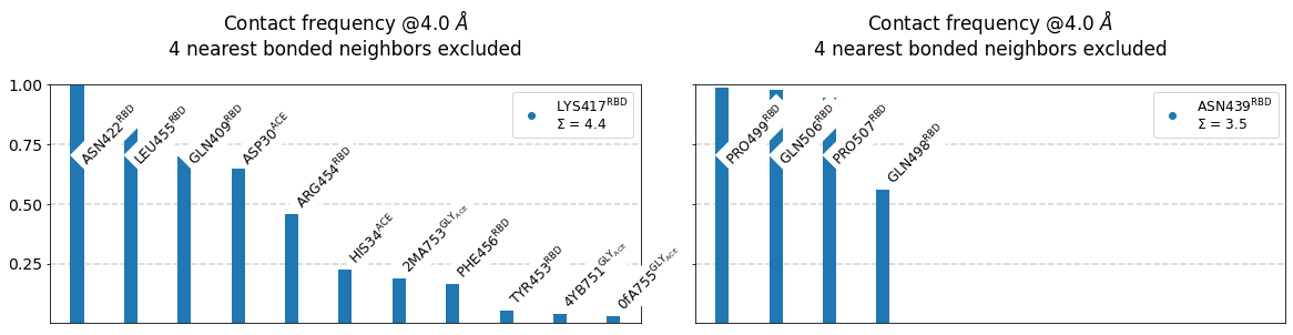
#idx freq contact fragments res_idxs ctc_idx Sum
1: 1.00 LYS417-ASN422 0-0 85-90 21 1.00
2: 0.93 LYS417-LEU455 0-0 85-123 30 1.93
3: 0.70 LYS417-GLN409 0-0 85-77 17 2.63
4: 0.65 LYS417-ASP30 0-2 85-218 83 3.28
5: 0.46 LYS417-ARG454 0-0 85-122 29 3.73
6: 0.22 LYS417-HIS34 0-2 85-222 87 3.96
7: 0.19 LYS417-2MA753 0-3 85-929 105 4.14
8: 0.16 LYS417-PHE456 0-0 85-124 31 4.31
9: 0.05 LYS417-TYR453 0-0 85-121 28 4.36
10: 0.04 LYS417-4YB751 0-3 85-927 103 4.40
11: 0.03 LYS417-0fA755 0-3 85-931 107 4.43
These 11 contacts capture 4.43 (~99%) of the total frequency 4.47 (over 108 input contacts)
#idx freq contact fragments res_idxs ctc_idx Sum
1: 0.99 ASN439-PRO499 0-0 107-167 142 0.99
2: 0.98 ASN439-GLN506 0-0 107-174 149 1.97
3: 0.95 ASN439-PRO507 0-0 107-175 150 2.91
4: 0.56 ASN439-GLN498 0-0 107-166 141 3.48
These 4 contacts capture 3.48 (~100%) of the total frequency 3.48 (over 71 input contacts)
After we have computed the per-residue neighborhoods, the next cell is just some reordering of the data into more practical, per-residue dictionaries:
[6]:
neighborhoods = {key : neighborhoods[key] for key in ['WT', 'K417V', 'N439K','N439K/K417V']}
pos417 = {key:val[85] for key, val in neighborhoods.items()}
pos439 = {key:val[107] for key, val in neighborhoods.items()}
Before we continue, we can save the neighborhoods for later use, s.t. they don’t have to be computed every time:
[7]:
#np.save("pos417.npy",pos417)
#np.save("pos439.npy",pos439)
Plotting the Contact-Frequencies
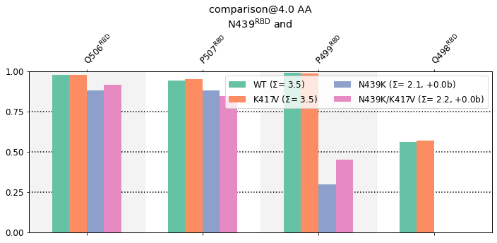
Next, we use mdciao.cli.compare plot the per-residue contact-frequencies of all four systems next to one another. The function call can be minimal or very customized, here we present some parameter values that yield the most informative plots:
[8]:
#pos417 = np.load("pos417.npy",allow_pickle=True)[()]
#pos439 = np.load("pos439.npy",allow_pickle=True)[()]
mdciao.cli.compare(pos417, ctc_cutoff_Ang=4,
mutations_dict={"V417": "K417",
"K439": "N439"
},
anchor="K417",
defrag=None,
width=.15,
lower_cutoff_val=.2,
fontsize=12,
legend_rows=2,
colors="Set2",
#distro=True,
#n_cols=3,
);
mdciao.cli.compare(pos439, ctc_cutoff_Ang=4,
mutations_dict={"V417": "K417",
"K439": "N439"
},
anchor="N439",
width=.15,
lower_cutoff_val=.2,
defrag=None,
fontsize=12,
legend_rows=2,
colors="Set2"
);
These interactions are not shared:
0LB752@GLY_ACE, 0fA755@GLY_ACE, 4YB751@GLY_ACE, A2753@GLY_ACE, D30@ACE, E406@RBD, F456@RBD
Their cumulative ctc freq is 2.94.
Created files
freq_comparison.pdf
freq_comparison.xlsx
These interactions are not shared:
Q325@ACE, Q498@RBD
Their cumulative ctc freq is 1.16.
Created files
freq_comparison.pdf
freq_comparison.xlsx
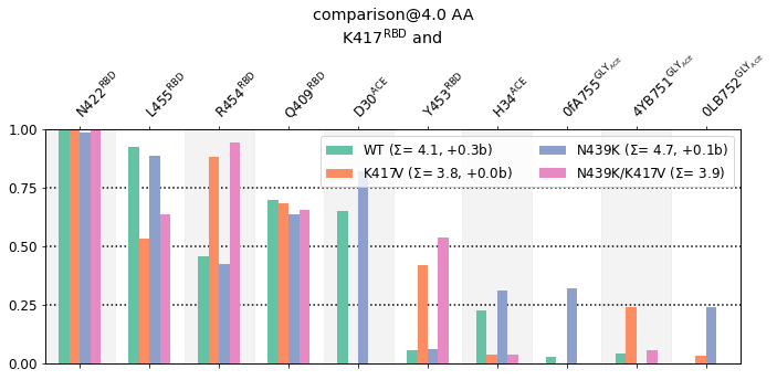
Some observations:
In the K417@RBD-neighborhood
The K417V mutants (single or double)
The N439K mutant doesn’t affect the K417@RBD neighborhood much (the green and blue bars are similar)
In the N439@RBD-neighborhood:
Distributions and Violin Plots
Frequencies with a hard cutoff (4 Angstrom, in this case) are reductive, and don’t tell the whole story, but allow for a compact overview a the large dataset (8K trajectories, 4 setups) in one plot per mutated residue, and already give an impression of the local changes around the mutated sites.
To get a cut-off independent comparison, we can use several mdciao-methods:
Use again
mdciao.cli.compare, but uncommenting thedistro=Trueparameter: For each residue neighborhood, this will produce a multi-panel figure (you can control its column-to-row form withn_cols) where each panel contains the distribution of one residue-residue distance for all systems:'WT', 'K417V', 'N439K','N439K/K417V'. The distributions are much more telling of the behaviour of the residue-residue distance, informing about it’s about it’s modes and spread.
Note
You also have to comment-out the lower_cutoff_val=.2 parameter.
Compact all the distributions into one single-panel, using violin-plots. The violins are simply the same distributions as above, only mirored (to get the nice, symmetric violins) and oriented vertically along the y-axis
Let’s try both options for the K417-neighborhood:
[9]:
mdciao.cli.compare(pos417, ctc_cutoff_Ang=4,
mutations_dict={"V417": "K417",
"K439": "N439"
},
anchor="K417",
defrag=None,
width=.15,
#lower_cutoff_val=.2,
fontsize=12,
legend_rows=2,
colors="Set2",
distro=True,
n_cols=3,
#sharex=True,
);
Created files
freq_comparison.pdf
freq_comparison.xlsx
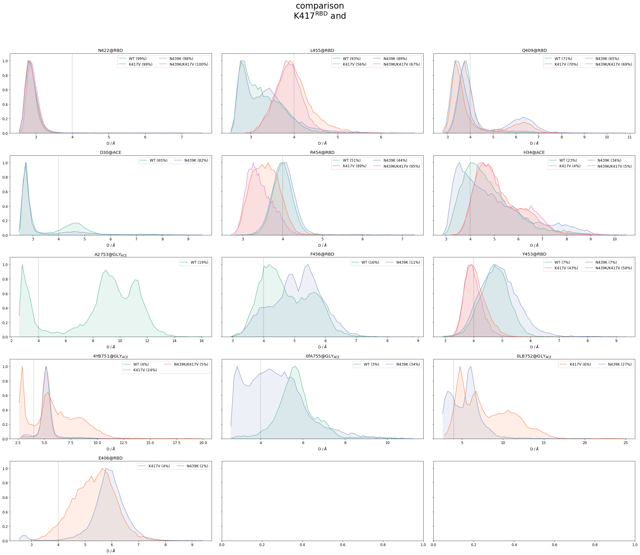
The multi-panel figure gives more detail about each residue-residue distance, but makes comparing accross distances a bit harder (even if you use the sharex=True parameter, which you should try).
Now we try the comparison via violin plots, using mdciao.plots.compare_violins:
[10]:
mdciao.plots.compare_violins(pos417,
ctc_cutoff_Ang=4,
figsize=(15,5),
colors="Set2",
defrag=None,
anchor="K417",
legend_rows=2,
mutations_dict={"V417": "K417",
"K439": "N439"
}
);
[10]:
(<Figure size 1080x360 with 1 Axes>,
<AxesSubplot:title={'center':'VAL417$^{\\mathrm{RBD}}$ neighborhood'}, ylabel='D / $\\AA$'>)
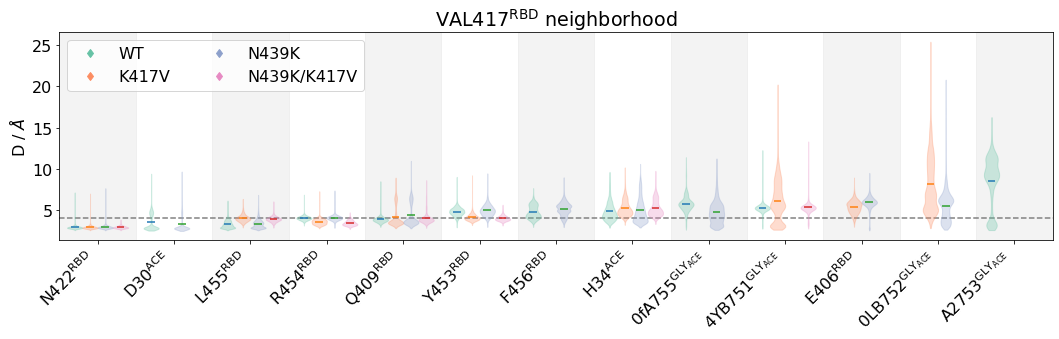
This plot is now more crowded but contains more information in one single panel, allowing to quickly differentiate the residue-residue distance-distributions, and the effect that the mutations have on them. We see how some of them remain compact, some are simply shifted, some are bimodal, have long tails etc.
Note
It’s a good exercise to compare the violins with the individual, per-contact panels from above and see that, indeed, the violins are just mirrored distributions.
Targeting Pre-Defined Sites
Wheareas the mdciao.cli.residue_neighborhoods creates a list of likely neighbors by using an initial, generous cutoff (15 Angstrom, in this case), we can also simply provide a list of residue-residue distances of interest, regardless of whether they’re likely neighbors or not. This has the advantage of reducing the number of overall residue-residue distances computed, but neglects anything not included in that list.
In mdciao, such a small(ish) group of contacts is called a site, and there’s an API-submodule to handle them as well as a CLI-method to compute them, mdciao.cli.sites.
To select these contacts of interest, we can use our observations of the frequency plots from above. We will focus on the contacts most impacted by the mutations, and put them into a site definition, which is just a python dictionary with some human-readable form.
Note
Although the word ``site`` somehow hints at the contacts being spatially close (like a binding site, or a motif, etc), this doesn’t have to be the case. ``site`` is just a label under which to group contacts.
In any case, you can pass a list of sites to the CLI and API methods if you prefer to break down a large(ish) list of contacts into several smaller ones.
Check mdciao.sites for more info on constructing sites, interactively or as .JSON files.
[11]:
my_site ={"name" :"changed contacts",
"pairs":{"AAresSeq":[
"K417-D30",
"K417-L455",
"K417-R454",
"K417-Y453",
"N439-P499",
"N439-Q498"
]}}
We do a little Python to make sure the above dictionary works with all mutants:
[12]:
from copy import deepcopy
my_sites_mut_adapted={}
for syskey in filename2system.values():
#print(syskey)
my_sites_mut_adapted[syskey]=deepcopy(my_site)
mutations_dict={}
#Only populate mutations_dict if needed
if syskey!="WT":
for mut in syskey.split("/"):
mutations_dict.update({mut[:4]:mut[-1]+mut[1:-1]})
# We use one of mdciao's str_and_dict method for recursive mutation
my_sites_mut_adapted[syskey]["pairs"]['AAresSeq']=[mdciao.utils.str_and_dict.replace_w_dict(pair,mutations_dict) for pair in my_sites_mut_adapted[syskey]["pairs"]["AAresSeq"]]
my_sites_mut_adapted
[12]:
{'N439K': {'name': 'changed contacts',
'pairs': {'AAresSeq': ['K417-D30',
'K417-L455',
'K417-R454',
'K417-Y453',
'K439-P499',
'K439-Q498']}},
'K417V': {'name': 'changed contacts',
'pairs': {'AAresSeq': ['V417-D30',
'V417-L455',
'V417-R454',
'V417-Y453',
'N439-P499',
'N439-Q498']}},
'N439K/K417V': {'name': 'changed contacts',
'pairs': {'AAresSeq': ['V417-D30',
'V417-L455',
'V417-R454',
'V417-Y453',
'K439-P499',
'K439-Q498']}},
'WT': {'name': 'changed contacts',
'pairs': {'AAresSeq': ['K417-D30',
'K417-L455',
'K417-R454',
'K417-Y453',
'N439-P499',
'N439-Q498']}}}
Now that we have per-setup site definitions, we simply iterate again over setups passing the corresponding site definition:
Note
simply means that a very simple call to the method would be enough. Below, we use the optional parameters to showcase some of the advanced functionality.
Computing the Sites
[13]:
sites = {}
for fn, syskey in filename2system.items():
print(syskey)
pattern = os.path.join(datadir,fn+"*.h5")
sites[syskey] = mdciao.cli.sites([my_sites_mut_adapted[syskey]],
pattern,
n_jobs=7,
ctc_cutoff_Ang=4,
fragment_names=["RBD","GLY_RBD","ACE","GLY_ACE","ions","ions"],
fragments=["chains"],
no_disk=True,
figures=False,
plot_timedep=False)["changed contacts"]
N439K
Will compute the sites
site dict with name changed contacts
in the trajectories:
/media/perezheg/6TB_HD/FAH_aws/strided/50/run0-clone0.stride.050.h5
/media/perezheg/6TB_HD/FAH_aws/strided/50/run0-clone1.stride.050.h5
/media/perezheg/6TB_HD/FAH_aws/strided/50/run0-clone2.stride.050.h5
/media/perezheg/6TB_HD/FAH_aws/strided/50/run0-clone3.stride.050.h5
/media/perezheg/6TB_HD/FAH_aws/strided/50/run0-clone4.stride.050.h5
/media/perezheg/6TB_HD/FAH_aws/strided/50/run0-clone5.stride.050.h5
/media/perezheg/6TB_HD/FAH_aws/strided/50/run0-clone6.stride.050.h5
/media/perezheg/6TB_HD/FAH_aws/strided/50/run0-clone7.stride.050.h5
/media/perezheg/6TB_HD/FAH_aws/strided/50/run0-clone8.stride.050.h5
/media/perezheg/6TB_HD/FAH_aws/strided/50/run0-clone9.stride.050.h5
/media/perezheg/6TB_HD/FAH_aws/strided/50/run0-clone10.stride.050.h5
/media/perezheg/6TB_HD/FAH_aws/strided/50/run0-clone11.stride.050.h5
/media/perezheg/6TB_HD/FAH_aws/strided/50/run0-clone12.stride.050.h5
/media/perezheg/6TB_HD/FAH_aws/strided/50/run0-clone13.stride.050.h5
/media/perezheg/6TB_HD/FAH_aws/strided/50/run0-clone14.stride.050.h5
...[long list: omitted 1970 items]...
/media/perezheg/6TB_HD/FAH_aws/strided/50/run0-clone1985.stride.050.h5
/media/perezheg/6TB_HD/FAH_aws/strided/50/run0-clone1986.stride.050.h5
/media/perezheg/6TB_HD/FAH_aws/strided/50/run0-clone1987.stride.050.h5
/media/perezheg/6TB_HD/FAH_aws/strided/50/run0-clone1988.stride.050.h5
/media/perezheg/6TB_HD/FAH_aws/strided/50/run0-clone1989.stride.050.h5
/media/perezheg/6TB_HD/FAH_aws/strided/50/run0-clone1990.stride.050.h5
/media/perezheg/6TB_HD/FAH_aws/strided/50/run0-clone1991.stride.050.h5
/media/perezheg/6TB_HD/FAH_aws/strided/50/run0-clone1992.stride.050.h5
/media/perezheg/6TB_HD/FAH_aws/strided/50/run0-clone1993.stride.050.h5
/media/perezheg/6TB_HD/FAH_aws/strided/50/run0-clone1994.stride.050.h5
/media/perezheg/6TB_HD/FAH_aws/strided/50/run0-clone1995.stride.050.h5
/media/perezheg/6TB_HD/FAH_aws/strided/50/run0-clone1996.stride.050.h5
/media/perezheg/6TB_HD/FAH_aws/strided/50/run0-clone1997.stride.050.h5
/media/perezheg/6TB_HD/FAH_aws/strided/50/run0-clone1998.stride.050.h5
/media/perezheg/6TB_HD/FAH_aws/strided/50/run0-clone1999.stride.050.h5
with a stride of 1 frames.
Using method 'chains' these fragments were found
fragment 0 with 196 AAs ACE332 ( 0) - NME527 (195 ) (0)
fragment 1 with 10 AAs UYB729 ( 196) - 0fA738 (205 ) (1)
fragment 2 with 709 AAs ACE18 ( 206) - NME726 (914 ) (2)
fragment 3 with 58 AAs UYB739 ( 915) - 0fA796 (972 ) (3)
fragment 4 with 2 AAs CL973 ( 973) - ZN1 (974 ) (4) resSeq jumps
fragment 5 with 365 AAs Na+976 ( 975) - Na+1340 (1339) (5)
residue residx fragment resSeq BW CGN
LYS417 85 0 85 None None
LYS439 107 0 107 None None
TYR453 121 0 121 None None
ARG454 122 0 122 None None
LEU455 123 0 123 None None
GLN498 166 0 166 None None
PRO499 167 0 167 None None
ASP30 218 2 218 None None
freq label residue idxs sum
0 0.82 K417@RBD - D30@ACE 85 218 0.82
1 0.89 K417@RBD - L455@RBD 85 123 1.71
2 0.42 K417@RBD - R454@RBD 85 122 2.13
3 0.06 K417@RBD - Y453@RBD 85 121 2.19
4 0.30 K439@RBD - P499@RBD 107 167 2.49
5 0.00 K439@RBD - Q498@RBD 107 166 2.49
K417V
Will compute the sites
site dict with name changed contacts
in the trajectories:
/media/perezheg/6TB_HD/FAH_aws/strided/50/run1-clone0.stride.050.h5
/media/perezheg/6TB_HD/FAH_aws/strided/50/run1-clone1.stride.050.h5
/media/perezheg/6TB_HD/FAH_aws/strided/50/run1-clone2.stride.050.h5
/media/perezheg/6TB_HD/FAH_aws/strided/50/run1-clone3.stride.050.h5
/media/perezheg/6TB_HD/FAH_aws/strided/50/run1-clone4.stride.050.h5
/media/perezheg/6TB_HD/FAH_aws/strided/50/run1-clone5.stride.050.h5
/media/perezheg/6TB_HD/FAH_aws/strided/50/run1-clone6.stride.050.h5
/media/perezheg/6TB_HD/FAH_aws/strided/50/run1-clone7.stride.050.h5
/media/perezheg/6TB_HD/FAH_aws/strided/50/run1-clone8.stride.050.h5
/media/perezheg/6TB_HD/FAH_aws/strided/50/run1-clone9.stride.050.h5
/media/perezheg/6TB_HD/FAH_aws/strided/50/run1-clone10.stride.050.h5
/media/perezheg/6TB_HD/FAH_aws/strided/50/run1-clone11.stride.050.h5
/media/perezheg/6TB_HD/FAH_aws/strided/50/run1-clone12.stride.050.h5
/media/perezheg/6TB_HD/FAH_aws/strided/50/run1-clone13.stride.050.h5
/media/perezheg/6TB_HD/FAH_aws/strided/50/run1-clone14.stride.050.h5
...[long list: omitted 1968 items]...
/media/perezheg/6TB_HD/FAH_aws/strided/50/run1-clone1985.stride.050.h5
/media/perezheg/6TB_HD/FAH_aws/strided/50/run1-clone1986.stride.050.h5
/media/perezheg/6TB_HD/FAH_aws/strided/50/run1-clone1987.stride.050.h5
/media/perezheg/6TB_HD/FAH_aws/strided/50/run1-clone1988.stride.050.h5
/media/perezheg/6TB_HD/FAH_aws/strided/50/run1-clone1989.stride.050.h5
/media/perezheg/6TB_HD/FAH_aws/strided/50/run1-clone1990.stride.050.h5
/media/perezheg/6TB_HD/FAH_aws/strided/50/run1-clone1991.stride.050.h5
/media/perezheg/6TB_HD/FAH_aws/strided/50/run1-clone1992.stride.050.h5
/media/perezheg/6TB_HD/FAH_aws/strided/50/run1-clone1993.stride.050.h5
/media/perezheg/6TB_HD/FAH_aws/strided/50/run1-clone1994.stride.050.h5
/media/perezheg/6TB_HD/FAH_aws/strided/50/run1-clone1995.stride.050.h5
/media/perezheg/6TB_HD/FAH_aws/strided/50/run1-clone1996.stride.050.h5
/media/perezheg/6TB_HD/FAH_aws/strided/50/run1-clone1997.stride.050.h5
/media/perezheg/6TB_HD/FAH_aws/strided/50/run1-clone1998.stride.050.h5
/media/perezheg/6TB_HD/FAH_aws/strided/50/run1-clone1999.stride.050.h5
with a stride of 1 frames.
Using method 'chains' these fragments were found
fragment 0 with 196 AAs ACE332 ( 0) - NME527 (195 ) (0)
fragment 1 with 10 AAs UYB729 ( 196) - 0fA738 (205 ) (1)
fragment 2 with 709 AAs ACE18 ( 206) - NME726 (914 ) (2)
fragment 3 with 58 AAs UYB739 ( 915) - 0fA796 (972 ) (3)
fragment 4 with 2 AAs CL973 ( 973) - ZN1 (974 ) (4) resSeq jumps
fragment 5 with 367 AAs Na+976 ( 975) - Na+1342 (1341) (5)
residue residx fragment resSeq BW CGN
VAL417 85 0 85 None None
ASN439 107 0 107 None None
TYR453 121 0 121 None None
ARG454 122 0 122 None None
LEU455 123 0 123 None None
GLN498 166 0 166 None None
PRO499 167 0 167 None None
ASP30 218 2 218 None None
freq label residue idxs sum
0 0.00 V417@RBD - D30@ACE 85 218 0.00
1 0.53 V417@RBD - L455@RBD 85 123 0.53
2 0.88 V417@RBD - R454@RBD 85 122 1.41
3 0.42 V417@RBD - Y453@RBD 85 121 1.83
4 0.99 N439@RBD - P499@RBD 107 167 2.82
5 0.57 N439@RBD - Q498@RBD 107 166 3.39
N439K/K417V
Will compute the sites
site dict with name changed contacts
in the trajectories:
/media/perezheg/6TB_HD/FAH_aws/strided/50/run2-clone0.stride.050.h5
/media/perezheg/6TB_HD/FAH_aws/strided/50/run2-clone1.stride.050.h5
/media/perezheg/6TB_HD/FAH_aws/strided/50/run2-clone2.stride.050.h5
/media/perezheg/6TB_HD/FAH_aws/strided/50/run2-clone3.stride.050.h5
/media/perezheg/6TB_HD/FAH_aws/strided/50/run2-clone4.stride.050.h5
/media/perezheg/6TB_HD/FAH_aws/strided/50/run2-clone5.stride.050.h5
/media/perezheg/6TB_HD/FAH_aws/strided/50/run2-clone6.stride.050.h5
/media/perezheg/6TB_HD/FAH_aws/strided/50/run2-clone7.stride.050.h5
/media/perezheg/6TB_HD/FAH_aws/strided/50/run2-clone8.stride.050.h5
/media/perezheg/6TB_HD/FAH_aws/strided/50/run2-clone9.stride.050.h5
/media/perezheg/6TB_HD/FAH_aws/strided/50/run2-clone10.stride.050.h5
/media/perezheg/6TB_HD/FAH_aws/strided/50/run2-clone11.stride.050.h5
/media/perezheg/6TB_HD/FAH_aws/strided/50/run2-clone12.stride.050.h5
/media/perezheg/6TB_HD/FAH_aws/strided/50/run2-clone13.stride.050.h5
/media/perezheg/6TB_HD/FAH_aws/strided/50/run2-clone14.stride.050.h5
...[long list: omitted 1970 items]...
/media/perezheg/6TB_HD/FAH_aws/strided/50/run2-clone1985.stride.050.h5
/media/perezheg/6TB_HD/FAH_aws/strided/50/run2-clone1986.stride.050.h5
/media/perezheg/6TB_HD/FAH_aws/strided/50/run2-clone1987.stride.050.h5
/media/perezheg/6TB_HD/FAH_aws/strided/50/run2-clone1988.stride.050.h5
/media/perezheg/6TB_HD/FAH_aws/strided/50/run2-clone1989.stride.050.h5
/media/perezheg/6TB_HD/FAH_aws/strided/50/run2-clone1990.stride.050.h5
/media/perezheg/6TB_HD/FAH_aws/strided/50/run2-clone1991.stride.050.h5
/media/perezheg/6TB_HD/FAH_aws/strided/50/run2-clone1992.stride.050.h5
/media/perezheg/6TB_HD/FAH_aws/strided/50/run2-clone1993.stride.050.h5
/media/perezheg/6TB_HD/FAH_aws/strided/50/run2-clone1994.stride.050.h5
/media/perezheg/6TB_HD/FAH_aws/strided/50/run2-clone1995.stride.050.h5
/media/perezheg/6TB_HD/FAH_aws/strided/50/run2-clone1996.stride.050.h5
/media/perezheg/6TB_HD/FAH_aws/strided/50/run2-clone1997.stride.050.h5
/media/perezheg/6TB_HD/FAH_aws/strided/50/run2-clone1998.stride.050.h5
/media/perezheg/6TB_HD/FAH_aws/strided/50/run2-clone1999.stride.050.h5
with a stride of 1 frames.
Using method 'chains' these fragments were found
fragment 0 with 196 AAs ACE332 ( 0) - NME527 (195 ) (0)
fragment 1 with 10 AAs UYB729 ( 196) - 0fA738 (205 ) (1)
fragment 2 with 709 AAs ACE18 ( 206) - NME726 (914 ) (2)
fragment 3 with 58 AAs UYB739 ( 915) - 0fA796 (972 ) (3)
fragment 4 with 2 AAs CL973 ( 973) - ZN1 (974 ) (4) resSeq jumps
fragment 5 with 366 AAs Na+976 ( 975) - Na+1341 (1340) (5)
residue residx fragment resSeq BW CGN
VAL417 85 0 85 None None
LYS439 107 0 107 None None
TYR453 121 0 121 None None
ARG454 122 0 122 None None
LEU455 123 0 123 None None
GLN498 166 0 166 None None
PRO499 167 0 167 None None
ASP30 218 2 218 None None
freq label residue idxs sum
0 0.00 V417@RBD - D30@ACE 85 218 0.00
1 0.64 V417@RBD - L455@RBD 85 123 0.64
2 0.95 V417@RBD - R454@RBD 85 122 1.59
3 0.54 V417@RBD - Y453@RBD 85 121 2.12
4 0.45 K439@RBD - P499@RBD 107 167 2.57
5 0.00 K439@RBD - Q498@RBD 107 166 2.57
WT
Will compute the sites
site dict with name changed contacts
in the trajectories:
/media/perezheg/6TB_HD/FAH_aws/strided/50/run3-clone0.stride.050.h5
/media/perezheg/6TB_HD/FAH_aws/strided/50/run3-clone1.stride.050.h5
/media/perezheg/6TB_HD/FAH_aws/strided/50/run3-clone2.stride.050.h5
/media/perezheg/6TB_HD/FAH_aws/strided/50/run3-clone3.stride.050.h5
/media/perezheg/6TB_HD/FAH_aws/strided/50/run3-clone4.stride.050.h5
/media/perezheg/6TB_HD/FAH_aws/strided/50/run3-clone5.stride.050.h5
/media/perezheg/6TB_HD/FAH_aws/strided/50/run3-clone6.stride.050.h5
/media/perezheg/6TB_HD/FAH_aws/strided/50/run3-clone7.stride.050.h5
/media/perezheg/6TB_HD/FAH_aws/strided/50/run3-clone8.stride.050.h5
/media/perezheg/6TB_HD/FAH_aws/strided/50/run3-clone9.stride.050.h5
/media/perezheg/6TB_HD/FAH_aws/strided/50/run3-clone10.stride.050.h5
/media/perezheg/6TB_HD/FAH_aws/strided/50/run3-clone11.stride.050.h5
/media/perezheg/6TB_HD/FAH_aws/strided/50/run3-clone12.stride.050.h5
/media/perezheg/6TB_HD/FAH_aws/strided/50/run3-clone13.stride.050.h5
/media/perezheg/6TB_HD/FAH_aws/strided/50/run3-clone14.stride.050.h5
...[long list: omitted 1970 items]...
/media/perezheg/6TB_HD/FAH_aws/strided/50/run3-clone1985.stride.050.h5
/media/perezheg/6TB_HD/FAH_aws/strided/50/run3-clone1986.stride.050.h5
/media/perezheg/6TB_HD/FAH_aws/strided/50/run3-clone1987.stride.050.h5
/media/perezheg/6TB_HD/FAH_aws/strided/50/run3-clone1988.stride.050.h5
/media/perezheg/6TB_HD/FAH_aws/strided/50/run3-clone1989.stride.050.h5
/media/perezheg/6TB_HD/FAH_aws/strided/50/run3-clone1990.stride.050.h5
/media/perezheg/6TB_HD/FAH_aws/strided/50/run3-clone1991.stride.050.h5
/media/perezheg/6TB_HD/FAH_aws/strided/50/run3-clone1992.stride.050.h5
/media/perezheg/6TB_HD/FAH_aws/strided/50/run3-clone1993.stride.050.h5
/media/perezheg/6TB_HD/FAH_aws/strided/50/run3-clone1994.stride.050.h5
/media/perezheg/6TB_HD/FAH_aws/strided/50/run3-clone1995.stride.050.h5
/media/perezheg/6TB_HD/FAH_aws/strided/50/run3-clone1996.stride.050.h5
/media/perezheg/6TB_HD/FAH_aws/strided/50/run3-clone1997.stride.050.h5
/media/perezheg/6TB_HD/FAH_aws/strided/50/run3-clone1998.stride.050.h5
/media/perezheg/6TB_HD/FAH_aws/strided/50/run3-clone1999.stride.050.h5
with a stride of 1 frames.
Using method 'chains' these fragments were found
fragment 0 with 196 AAs ACE332 ( 0) - NME527 (195 ) (0)
fragment 1 with 10 AAs UYB729 ( 196) - 0fA738 (205 ) (1)
fragment 2 with 709 AAs ACE18 ( 206) - NME726 (914 ) (2)
fragment 3 with 58 AAs UYB739 ( 915) - 0fA796 (972 ) (3)
fragment 4 with 2 AAs CL973 ( 973) - ZN1 (974 ) (4) resSeq jumps
fragment 5 with 366 AAs Na+976 ( 975) - Na+1341 (1340) (5)
residue residx fragment resSeq BW CGN
LYS417 85 0 85 None None
ASN439 107 0 107 None None
TYR453 121 0 121 None None
ARG454 122 0 122 None None
LEU455 123 0 123 None None
GLN498 166 0 166 None None
PRO499 167 0 167 None None
ASP30 218 2 218 None None
freq label residue idxs sum
0 0.65 K417@RBD - D30@ACE 85 218 0.65
1 0.93 K417@RBD - L455@RBD 85 123 1.58
2 0.46 K417@RBD - R454@RBD 85 122 2.03
3 0.05 K417@RBD - Y453@RBD 85 121 2.09
4 0.99 N439@RBD - P499@RBD 107 167 3.08
5 0.56 N439@RBD - Q498@RBD 107 166 3.64
We can also save the sites for later use:
[14]:
#np.save("sites.npy",sites)
Reporting the Sites
Finally, we can use again the compare-method of mdciao to see the impact of the mutations on the site. Since the overall number of computed distances is much smaller, we can use the distro==True and get much more information on the distances without having a large figure:
[15]:
#sites = np.load("sites.npy",allow_pickle=True)[()]
mdciao.cli.compare(sites, distro=True,
n_cols=2,
mutations_dict={"V417": "K417",
"K439": "N439"
},
sharex=True,
ctc_cutoff_Ang=4,
colors="Set2");
Created files
freq_comparison.pdf
freq_comparison.xlsx
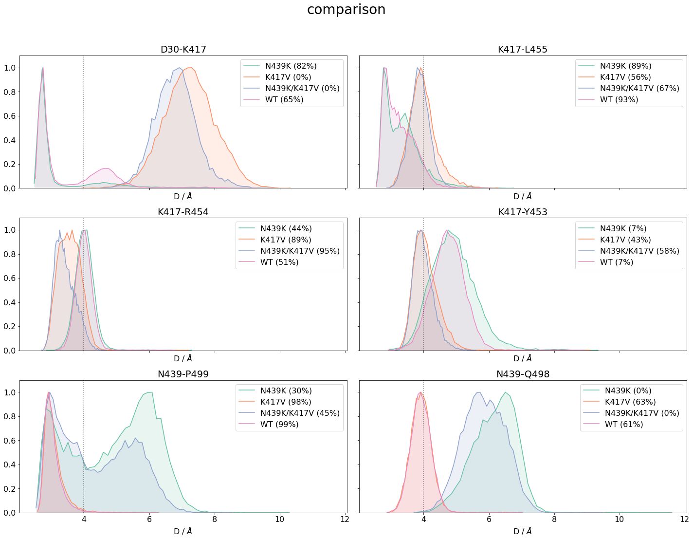
We see the effects mentioned before about the disruption of salt-bridges by e.g. with D30, in the upper left panel. We also notice that the frequencies reported in the legend coincide with those initially reported in the bar plots at the very top of this page.
Note
When comparing these distributions obtained via the site-method, with the distributions reported further up, both as per-contact panels or in the one-panel-for-all violin-plots, you’ll notice that some distributions are missing. Look, for example, at the the K417-D30 violins: two of them are missing.
This is per-design: when computing those residue neighborhoods using mdciao.cli.residue_neighborhoods, we specified ctc_cutoff_Ang = 4. This means that only those residues considered neighbors at a cutoff of 4 Angstrom are kept in the results. In the K417V mutants, the salt bridge with D30 is totally disrupted and never contributes to the frequency (only very
marginally), so it has been completely eliminated from the neighborhood.
site-methods, on the other hand, have a static list of target residue-pairs and report on them regardless of whether they contribute to the neighborhood or not. The ctc_cutoff_Ang is used only to inform on frequencies, but not to control what contacts are kept in the site.
Two last observations:
sites or neighborhoods are both ContactGroup-objects, and behave very similarly. A
ContactGroupismdciao’s class to handle groups of residue-residue distances.If you suspect that a residue-residue pair is missing from your figures and/or tables, please take a look at our FAQ: Missing Contacts.
3D Visualization
In future releases, we will include a method in the ContactGroup to automatically highlight it’s residues in an nglviewer widget. For now, we simply expose here how that method would look like:
[19]:
def show_neighborhood3D(self,iwd,ctc_cutoff_Ang=None, top=None, representation="licorice"):
if top is None:
assert isinstance(self.top, md.Topology)
if ctc_cutoff_Ang is None:
freqs = np.ones(self.n_ctcs)
else:
freqs = self.frequency_per_contact(ctc_cutoff_Ang)
if self.is_neighborhood:
anchor_ats = [aa.index for aa in self.top.residue(self.shared_anchor_residue_index).atoms]
atoms = []
for fr, pair in zip(freqs, self.res_idxs_pairs):
if fr >0:
for rr in pair:
atoms.extend([aa.index for aa in self.top.residue(rr).atoms])
[atoms.remove(aa) for aa in anchor_ats]
iwd.add_representation(representation, selection=atoms)
iwd.add_representation("ball_and_stick", selection=anchor_ats)
iwd.add_representation("spacefill", selection=anchor_ats)
iwd = nglview.show_mdtraj(md.load(os.path.join(datadir,"run3-clone0.stride.050.h5"))[0])
show_neighborhood3D(pos417["WT"],
iwd,
#representation="spacefill"
)
iwd
[ ]: